Finding a Learning Rate with Tensorflow 2

Choosing a good learning rate is the most important hyper-parameter choice when training a deep neural network (assuming a gradient based optimization algorithm is used).

Choosing a learning rate that's too small leads to extremely long training times. Whereas a learning rate that's too large might miss the optimum and lead to training divergence.

Fortunately there is a simple way to estimate a good learning rate. First described by Leslie Smith in Cyclical Learning Rates for Training Neural Networks, and then popularized by the FastAI library, which has a first class implementation of a learning rate finder.

The technique can be described as follows:

1. Start with a very low learning rate e.g. 1-e7.
2. After each batch, increase the learning rate and record the loss and learning rate.
3. Stop when a very high learning rate (10+) is reached, or the loss value explodes.
4. Plot the recorded losses and learning rates against each other and choose a learning rate where the loss is strictly decreasing at a rapid rate.

For a more thorough explanation of the technique see Sylvain Gugger's post.

Implementation

Implementing the technique in Tensorflow 2 is straightforward when implemented a Keras Callback. A Tensorflow 2 compatible implementation is given below and is also available on Github.

The implementation uses an exponentially increasing learning rate, which means smaller learning rate regions will be explored more thoroughly than larger learning rate regions.

The losses are also smoothed using a smoothing factor to prevent sudden or erratic changes in the loss (due to the stochastic nature of the training) from stopping the search process prematurely.

Application

In order to use the LRFinder: instantiate and compile a model, adding it as a callback. The model can then be fit as usual. The callback will record the losses and learning rates and stop training when the loss value diverges or the maximum learning rate is reached.

from tensorflow.keras.layers import Conv2D, MaxPool2D, Flatten, Dense, Dropout

def build_model():
    return tf.keras.models.Sequential([
        Conv2D(32, 3, activation='relu'),
        MaxPool2D(),
        Flatten(),
        Dense(128, activation='relu'),
        Dropout(0.1),
        Dense(10, activation='softmax')
    ])

lr_finder = LRFinder()
model = build_model()
model.compile(optimizer='adam', loss='sparse_categorical_crossentropy')
_ = model.fit(train_ds, epochs=5, callbacks=[lr_finder], verbose=False)

lr_finder.plot()

The plot method will produce a graph of the results, allowing visually choosing a learning rate:

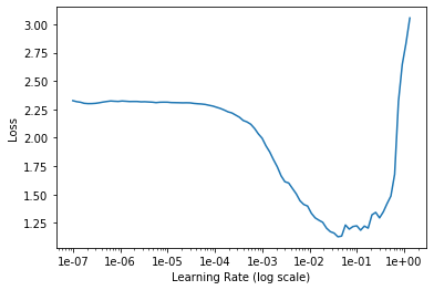
A value should be chosen in a region where the loss is rapidly, but strictly decreasing. Examples of such graphs and how they are interpreted are also available in previous posts.

It is important to rebuild and recompile the model after the LRFinder is used in order to reset the weights that were updated during the mock training run.

A complete example of how the LRFinder is applied is available in this Jupyter notebook.

References

1. Cyclical Learning Rates for Training Neural Networks, Leslie N. Smith
2. https://docs.fast.ai/callbacks.lr_finder.html
3. How Do You Find a Good Learning Rate, Sylvain Gugger