African Antelope: A Case Study of Creating an Image Dataset with FastAI

(Note: this post was updated on 2019-05-19 for clarity.)

In this post we will look at an end-to-end case study of how to creating and cleaning your own small image dataset from scratch and then train a ResNet convolutional neural network to classify the images using the FastAI library.

Besides gathering the data, we will also illustrate how to perform model assisted data cleaning to partially automate the cleaning of the data itself.

Contents

1. Creating an Image Dataset
   i.   Downloading the Data
   ii.  Cleaning the Data
2. Training the Model
   i.   Building the Dataset
   ii.  Creating the Model
   iii. Fitting the Model
   iv. Initial Results
3. Model Assisted Data Cleaning
4. Full Model Training
   i.   Results
5. Conclusion

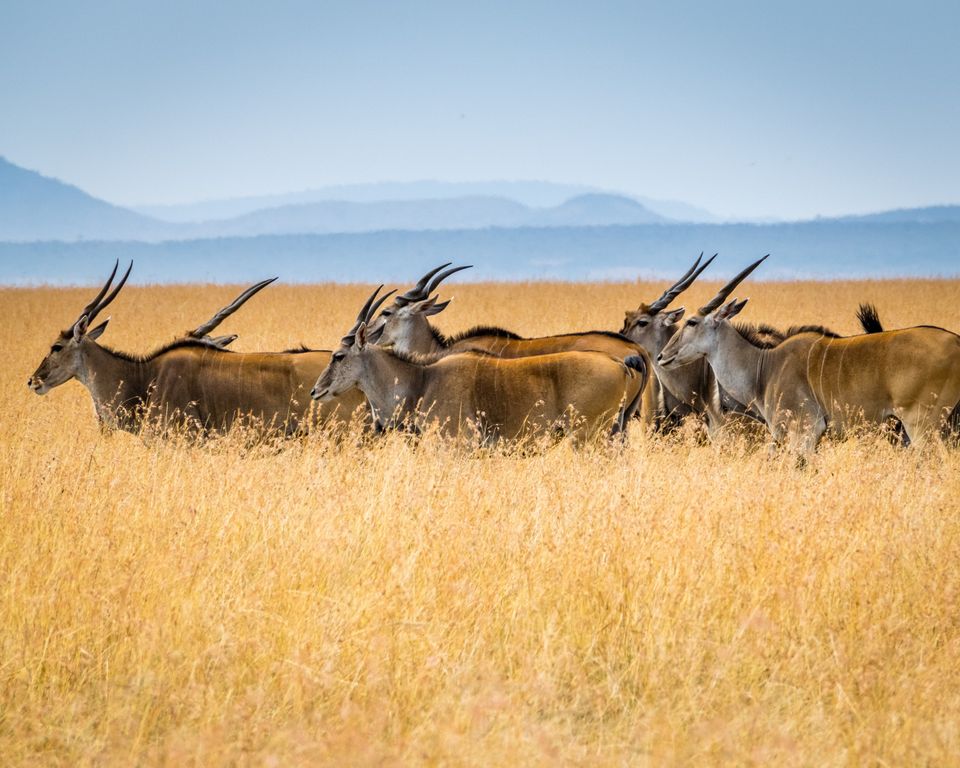
The classification problem we will be solving is the classification of major species of African antelope in the wild. The dataset we will create will consist of 13 African antelope species. As we will see this is an interesting challenge, as orientation, colour and very specific features of the antelope (e.g. the horns) are often necessary to distinguish each species. We will also see that it's not always necessary to have a very large dataset in order to use deep learning.

A Jupyter notebook and Python script with the complete code for the example is available on Github. In order to run the notebook or script, ensure you have a FastAI environment setup.

Creating an Image Dataset

We will start by downloading the images for our dataset. When creating your own dataset, carefully think of the use case you are building it for, and think of the type of images that are representative of the actual problem you are trying to solve.

In the case of antelope, there are a few things to consider:

• Male and female variants of the species have significant differences.
• We are interested in pictures of the animals in the wild as opposed to captivity.
• The young of each species could be very different from the adult.
• The colour of a species could be a distinguishing factor. For example, photos taken at dawn or dusk might not be appropriate.

In general try and think of any biases or specific contexts present in your subject matter that might not be applicable to the problem being solved.

Downloading the Data

In order to download the actual images, we will use google-images-download, an open source tool that can download images from Google Images based on keyword search.

The code to download the images is as follows:

def download_antelope_images(output_path: Path, limit: int = 50) -> None:
    """Download images for each of the antelope to the output path.
    
    Each species is put in a separate sub-directory under output_path.
    """
    response = google_images_download.googleimagesdownload()

    for antelope in ANTELOPE:
        for gender in ['male', 'female']:
            output_directory = str(output_path/antelope).replace(' ', '_')

            arguments = {
                'keywords': f'wild {antelope} {gender} -hunting -stock',
                'output_directory': output_directory,
                'usage_rights': 'labeled-for-nocommercial-reuse',
                'no_directory': True,
                'size': 'medium',
                'limit': limit
            }
            response.download(arguments)

The code above searches for images of each antelope species in the ANTELOPE list. For every species, we perform two searches: one for male examples and one for female examples. We add the keyword wild to look for examples of the antelope in the wild, while excluding the keywords hunting and stock to limit the search to images applicable to our use case. Also be sure to search for images with the appropriate usage rights.

The images are downloaded putting each species in a separate folder named for the species, thereby building an 'Imagenet-style' dataset. This is compatible with FastAI's ImageDataBunch.from_folder helper which will use to load the dataset for training.

The download was limited to 50 examples each for the male and female of each species.

Cleaning the Data

Even though Google does a very good job of finding the correct images for keyword searches, we still have to make sure the images are appropriate for our use case.

Unfortunately this is a time consuming process which is hard to automate (more on that later). Some checks can be automated, for instance, removing duplicates based on MD5 sums, or using the file names to check for labelling errors (as I do in the Python script). However, I still had to manually inspect the images, removing examples I considered inappropriate. These images mostly involved photos of multiple species in a single example, images of predators hunting or feasting on the antelope, man made illustrations of the antelope or antelopes in captivity.

After the data cleaning I was left with between 60 and 100 images (with an average of 85) per species. This is not a large dataset - we will however see that the deep learning model still performs very well.

Training the Model

With the data prepared we can now build the training and validation datasets and train our model. We will be using transfer learning to train a ResNet model that is pre-trained on the ImageNet dataset.

Building the Dataset

FastAI makes use of DataBunch objects to group the training, validation and test datasets. The DataBunch object also makes sure the Pytorch DataLoader loads to the correct device (GPU/CPU) and supports applying image transforms for data augmentation. Further, the DataBunch normalizes the data using the ImageNet statistics, which is necessary, as the model is pre-trained on the ImageNet data. The ImageDataBunch can be created with:

image_data = ImageDataBunch.from_folder(DATA_PATH, valid_pct=VALID_PCT,\
                                            ds_tfms=get_transforms(),\
                                            size=IMAGE_SIZE,\
                                            bs=BATCH_SIZE)\
                                            .normalize(imagenet_stats)

We specify the percentage of the data to use for the validation set with VALID_PCT ( 0.2 or 20% in this case), the IMAGE_SIZE (224 for ImageNet trained models) and a BATCH_SIZE (32 for this example, but you can use a smaller or larger batch size, depending on how much VRAM your GPU has).

Creating the Model

Creating the ResNet model is very straightforward with FastAI. We use the cnn_learner helper method, specifying our ImageDataBunch and chosen ResNet architecture:

learn = cnn_learner(image_data, models.resnet50, metrics=[error_rate, accuracy])

Here we use a pre-trained resnet50 model from the Pytorch Torchvision library. If you have a smaller GPU, a pre-trained resnet34 works equally well.

We also specify the error_rate as a metric that will be calculated during training.

Fitting the Model

We are now ready to fit the model to our data. The initial training will only fine-tune the top fully-connected layers of the model; the other layer weights being frozen.

Before starting the training, we have to choose an appropriate learning rate, which is perhaps the single most important choice for effective training. FastAI provides the supremely useful lr_find method for this purpose, which is based on the technique discussed in Cyclical Learning Rates for Training Neural Networks.

learn.lr_find()
learn.recorder.plot()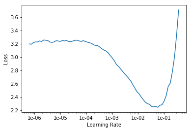

We when simply choose a learning rate (or range) where the loss is strictly decreasing. It's beneficial to choose the largest learning rate that has a decreasing loss, as this will speed up training.

Having chosen a learning rate range ( [1e-3, 1e-2] ) , we perform 5 training epochs using the 1cycle learning policy.

learn.fit_one_cycle(5, max_lr=slice(1e-3, 1e-2))
learn.save('stage-1')

epoch	train_loss	valid_loss	error_rate	time
0	1.352547	0.909331	0.281369	00:14
1	1.032153	0.774388	0.205323	00:13
2	0.737094	0.570336	0.178707	00:13
3	0.476649	0.451232	0.129278	00:13

epochtrain_lossvalid_losserror_ratetime01.3525470.9093310.28136900:1411.0321530.7743880.20532300:1320.7370940.5703360.17870700:1330.4766490.4512320.12927800:13

Initial Results

After the initial training we reach a validation accuracy of 87.07%. We can use FastAI's ClassificationInterpretation to further interpret the model's performance:

interp = ClassificationInterpretation.from_learner(learn)
interp.plot_confusion_matrix(figsize=(12,12), dpi=60)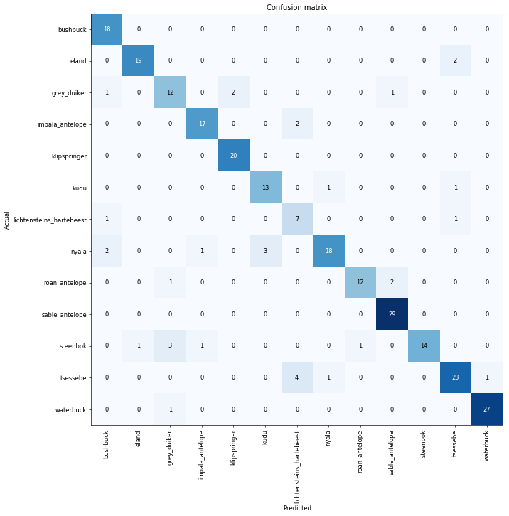

The interpreter also has a very useful feature that allows us to easily plot the the examples that had the largest loss values.

interp.plot_top_losses(9, figsize=(12,12))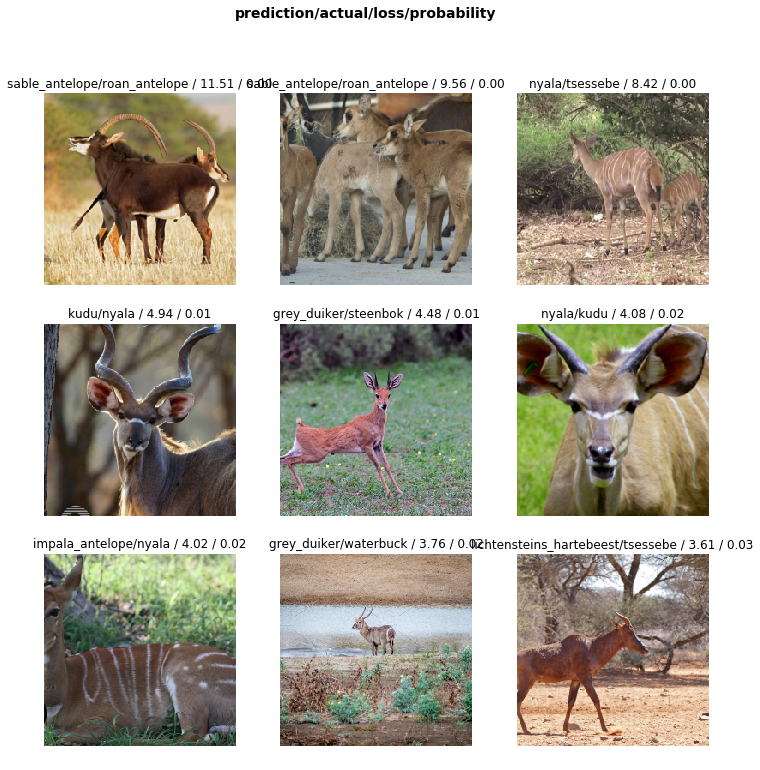

On issue seems to be images of close-up views of the antelope's face or photos where the antelope is not presented in the typical broadside view. In both these cases, distinguishing features such as patterns on the animal's coat or it's horns might be missing from the image. This highlights a potential flaw in how we gather the data: having many examples of one perspective of the subject matter, but neglecting other, valid perspectives.

Model Assisted Data Cleaning

The FastAI library provides an extremely useful Jupyter Notebook widget that aids in automating data clean-up by using the trained model itself: the ImageCleaner.

Using an ImageDataBunch, the dataset is then indexed by which images lead to the highest losses using the trained model. The ImageCleaner is then instantiated from the dataset and indices:

from fastai.widgets import *

images = (ImageList.from_folder(DATA_PATH)
                   .split_none()
                   .label_from_folder()
                   .transform(custom_transforms(), size=224)
                   .databunch())

ds, idxs = DatasetFormatter().from_toplosses(learn)

ImageCleaner(ds, idxs, DATA_PATH)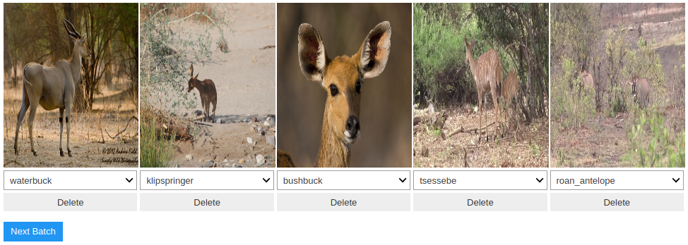

The widget then allows the you to remove images from the dataset or re-label the images in the case that images are incorrectly labelled.

Importantly, the ImageCleaner widget does not modify the data itself but instead creates a .csv file that contains the paths and labels of the cleaned data. We then need to construct an ImageDataBunch from the .csv file:

df = pd.read_csv(DATA_PATH/'cleaned.csv', header='infer')
image_data = (ImageDataBunch.from_df(DATA_PATH, df,
                                     valid_pct=VALID_PCT,
                                     ds_tfms=custom_transforms(),
                                     size=IMAGE_SIZE,
                                     bs=BATCH_SIZE)
              .normalize(imagenet_stats))

Full Model Training

Next we can look at training all the layers of the model instead of just the last, fully-connected layers. This is done by 'unfreezing' the other layers of the model before training.

We also have to find a new learning rate as the optimisation landscape has now completely changed:

learn.unfreeze()

learn.lr_find()
learn.recorder.plot()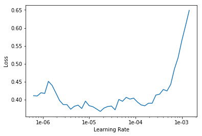

Finally, we fit the model again with the 1cycle policy for 20 epochs using a small learning rate:

learn.fit_one_cycle(20, max_lr=7e-5)

epoch	train_loss	valid_loss	error_rate	time
0	0.154993	0.311427	0.127962	00:14
1	0.185968	0.302535	0.127962	00:14
2	0.167942	0.291734	0.109005	00:14
3	0.181434	0.298713	0.094787	00:14
4	0.190612	0.400196	0.118483	00:14
5	0.209943	0.414060	0.118483	00:14
6	0.226450	0.462790	0.132701	00:14
7	0.248497	0.382834	0.113744	00:14
8	0.189046	0.343103	0.113744	00:14
9	0.141687	0.378920	0.132701	00:14
10	0.133787	0.400326	0.099526	00:14
11	0.136122	0.366274	0.109005	00:14
12	0.114380	0.343331	0.094787	00:14
13	0.091698	0.364937	0.109005	00:14
14	0.083694	0.331757	0.113744	00:14
15	0.069167	0.309694	0.104265	00:14
16	0.064571	0.312528	0.094787	00:14
17	0.057514	0.316830	0.085308	00:14
18	0.060952	0.323746	0.104265	00:14
19	0.057364	0.298466	0.085308	00:14

Results

Fitting all the layers of the neural network improves our training loss to 0.057 and our validation loss to 0.298 and increases our validation accuracy to 91.4692%.

Similar to earlier, we can create an interpreter and visualise our top losses:

interp = ClassificationInterpretation.from_learner(learn)
interp.plot_top_losses(9, figsize=(12,12), heatmap=True)

Here we pass the parameter heatmap=True to the plot_top_losses method, which will produce Grad-CAM (Gradient-weighted Class Activation Mapping) heatmaps for the images. Grad-CAM visualisations highlight the important regions in the image used for the prediction.

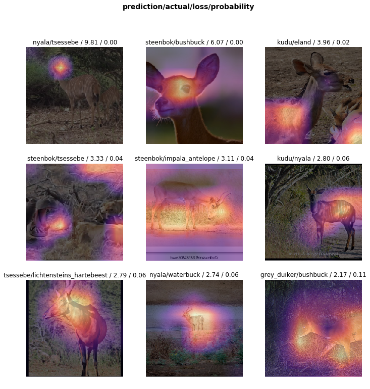
The Grad-CAM visualisations show that the model does however correctly identify the regions containing the antelope and confirms that it tends to focus on regions containing the body and horns of the antelope.

Finally we can calculate our final F1 score, also making use of TTA (Test Time Augmentation). TTA applies the same augmenting transforms we used during training when making a prediction. The actual prediction is then the average of the predictions over the transformations of an example, increasing the chance the model makes the correct prediction.

preds, targets = learn.TTA()
predicted_classes = np.argmax(preds, axis=1)

f1_score(targets, predicted_classes, average='micro')

0.9004739336492891

We end up with a final F1 score of 0.9.

Further Improvements

There are number of things we can investigate to further improve the model performance:

• More data could be gathered, especially of specific edge cases the model is struggling with: front and rear views of the animals and close-ups of antelope faces.
• Validate the transformations used to augment the dataset, especially colour distortion and image rotation/cropping. Some very specific features are sometimes required to distinguish one species from another and as such we have to ensure the transformations we use doesn't discard this information.
• Alternative architectures should be investigated that might perform better with the specific use case.

Conclusion

In this post we covered an end-to-end example of creating our own image dataset and using transfer learning to create an accurate deep learning image classifier for African antelope species. Our ResNet50 model reached an F1 score of 0.9 after only 24 epochs of training on roughly 880 examples spread over the 13 classes.

Unsurprisingly the hardest and most time consuming part of the deep learning exercise was not training the model, indeed the FastAI code to do so is only 5 lines long:

image_data = ImageDataBunch.from_folder(DATA_PATH, valid_pct=VALID_PCT,\
                                            ds_tfms=get_transforms(),\
                                            size=IMAGE_SIZE,\
                                            bs=BATCH_SIZE)\
                                            .normalize(imagenet_stats)

learner = cnn_learner(image_data, architecture, metrics=error_rate)
learner.fit_one_cycle(5, max_lr=slice(1e-3, 1e-2))
learner.unfreeze()
learner.fit_one_cycle(5, 1e-4)

Instead, the most difficult part is gathering and cleaning the data. Manual inspection of the data is tedious and time consuming, and still resulted in some problems slipping through.

However, we also demonstrated how to use the model itself to aid in cleaning the dataset using the ImageCleaner widget from the FastAI library.

Furthermore, we found that the dataset is not fully representative of the problem we are trying to solve, as the dataset is missing examples of some valid perspectives we might encounter in the real world.

There is no simple solution to creating a high quality and error free dataset (which is why open data initiatives are so valuable). However, an alternative to creating your own dataset is to find a dataset similar to a dataset you would need to solve your problem and then modifying it. In this case, we could have started with a dataset such as the Snapshot Serengeti dataset and used only images of antelope contained therein. An exercise left for next time.