An Overview of LightGBM

Contents

1. LightGBM Introduction
2. Gradient Boosting
   i. Algorithm
3. LightGBM API
   i. Plotting
   ii. Saving the model
4. LightGBM Parameters
   i. Tree parameters
   ii. Tuning for imbalanced data
   iii. Tuning for overfitting
   iv. Tuning for accuracy
5. Resources

Although maybe not as fashionable as deep learning algorithms in 2018, the effectiveness of tree and tree ensemble based learning methods certainly cannot be questioned. Across a variety of domains (restaurant visitor forecasting, music recommendation, safe driver prediction, and many more), ensemble tree models - specifically gradient boosted trees - are widely used on Kaggle, often as part of the winning solution.

Decision trees also have certain advantages over deep learning methods: decision trees are more readily interpreted than deep neural networks, naturally better at learning from imbalanced data, often much faster to train, and work directly with un-encoded feature data (such as text).

This post gives an overview of LightGBM and aims to serve as a practical reference. A brief introduction to gradient boosting is given, followed by a look at the LightGBM API and algorithm parameters. The examples given in this post are taken from an end-to-end practical example of applying LightGBM to the problem of credit card fraud detection: https://www.kaggle.com/avanwyk/a-lightgbm-overview.

LightGBM

LightGBM is an open-source framework for gradient boosted machines. By default LightGBM will train a Gradient Boosted Decision Tree (GBDT), but it also supports random forests, Dropouts meet Multiple Additive Regression Trees (DART), and Gradient Based One-Side Sampling (Goss).

The framework is fast and was designed for distributed training. It supports large-scale datasets and training on the GPU. In many cases LightGBM has been found to be more accurate and faster than XGBoost, though this is problem dependent.

Both LightGBM and XGBoost are widely used and provide highly optimized, scalable and fast implementations of gradient boosted machines (GBMs). I have previously used XGBoost for a number of applications, but have yet to take an in depth look at LightGBM.

The section below gives some theoretical background on gradient boosting. The section LightGBM API continues with practicalities on using the LightGBM.

Gradient Boosting

When considering ensemble learning, there are two primary methods: bagging and boosting. Bagging involves the training of many independent models and combines their predictions through some form of aggregation (averaging, voting etc.). An example of a bagging ensemble is a Random Forest.

Boosting instead trains models sequentially, where each model learns from the errors of the previous model. Starting with a weak base model, models are trained iteratively, each adding to the prediction of the previous model to produce a strong overall prediction.

In the case of gradient boosted decision trees, successive models are found by applying gradient descent in the direction of the average gradient, calculated with respect to the error residuals of the loss function, of the leaf nodes of previous models.

An excellent explanation of gradient boosting is given by Ben Gorman over on the Kaggle Blog and I strongly advise reading the post if you would like to understand gradient boosting. A summary is given here.

Considering decision trees, we proceed as follows. We start with an initial fit, \(F_0\), of our data: a constant value that minimizes our loss function \(L\):
$$ F_0(x) = \underset{\gamma}{arg\ \min} \sum^{n}_{i=1} L(y_i, \gamma) $$
in the case of optimizing the mean square error, we can take the mean of the target values:
$$ F_0(x) = \frac{1}{n} \sum^{n}_{i=1} y_i $$

With our initial guess of \(F_0\), we can now calculate the gradient, or pseudo residuals, of \(L\) with respect to \(F_0\):
$$ r_{i1} = -\frac{\partial L(y_i, F_{0}(x_i))}{\partial F_{0}(x_i)} $$

We now fit a decision tree \(h_{1}(x)\), to the residuals. Using a regression tree, this will yield the average gradient for each of the leaf nodes.

Now we can apply gradient descent to minimize the loss for each leaf by stepping in the direction of the average gradient for the leaf nodes as contained in our decision tree \(h_{1}(x)\). The step size is determined by a multiplier \(\gamma_{1}\) which can be optimized by performing a line search. The step size is further shrinked using a learning rate \(\lambda_{1}\), thus yielding a new boosted fit of the data:
$$ F_{1}(x) = F_{0}(x) + \lambda_1 \gamma_1 h_1(x) $$

Algorithm

Putting it all together, we have the following algorithm. For a number of boosting rounds \(M\) and a differentiable loss function \(L\):

Let \( F_0(x) = \underset{\gamma}{arg\ \min} \sum^{n}_{i=1} L(y_i, \gamma) \)
For m = 1 to M:

1. Calculate the pseudo residuals \( r_{im} = -\frac{\partial L(y_i, F_{m-1}(x_i))}{\partial F_{m-1}(x_i)} \)
2. Fit decision tree \( h_m(x) \) to \( r_{im} \)
3. Compute the step multiplier \( \gamma_m \) for each leaf of \( h_m(x) \)
4. Let \( F_m(x) = F_{m-1}(x) + \lambda_m \gamma_m h_m(x) \), where \( \lambda_m \) is the learning rate for iteration \(m\)

One caveat of the above explanation is that it neglects to incorporate a regularization term in the loss function. An overview of the gradient boosting as given in the XGBoost documentation pays special attention to the regularization term while deriving the objective function.

In terms of LightGBM specifically, a detailed overview of the LightGBM algorithm and its innovations is given in the NIPS paper.

LightGBM API

Fortunately the details of the gradient boosting algorithm are well abstracted by LightGBM, and using the library is very straightforward.

LightGBM requires you to wrap datasets in a LightGBM Dataset object:

lgb_train = lgb.Dataset(X_train, y_train, free_raw_data=False)
lgb_val = lgb.Dataset(X_val, y_val, reference=lgb_train, free_raw_data=False)

The parameter free_raw_data controls whether the input data is freed after constructing the inner datasets.

LightGBM supports many parameters that control various aspects of the algorithm (more on that below). Some core parameters that should be defined are:

core_params = {
    'boosting_type': 'gbdt', # rf, dart, goss
    'objective': 'binary', # regression, multiclass, binary
    'learning_rate': 0.05,
    'num_leaves': 31,
    'nthread': 4,
    'metric': 'auc' # binary_logloss, mse, mae
}

We can then call the training API to train a model, specifying the number of boosting rounds and early stopping rounds as needed:

evals_result = {}
gbm = lgb.train(core_params, # parameter dict to use
                training_set,
                init_model=init_gbm, # enables continuous training.
                num_boost_round=boost_rounds, # number of boosting rounds.
                early_stopping_rounds=early_stopping_rounds,
                valid_sets=validation_set,
                evals_result=evals_result, # stores validation results.
                verbose_eval=False) # print evaluations during training.

Early stopping occurs when there is no improvement in either the objective evaluations or the metrics we defined as calculated on the validation data.

LightGBM also supports continuous training of a model through the init_model parameter, which can accept an already trained model.

A detailed overview of the Python API is available here.

Plotting

LightGBM has a built in plotting API which is useful for quickly plotting validation results and tree related figures.

Given the eval_result dictionary from training, we can easily plot validation metrics:

_ = lgb.plot_metric(evals)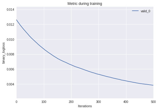

Another very useful features that contributes to the explainability of the tree is relative feature importance:

_ = lgb.plot_importance(model)

It is also possible to visualize individual trees:

_ = lgb.plot_tree(model, figsize=(20, 20))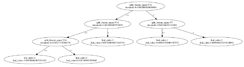

Saving the model

Models can easily be saved to a file or JSON:

gbm.save_model('cc_fraud_model.txt')

loaded_model = lgb.Booster(model_file='cc_fraud_model.txt')

# Output to JSON
model_json = gbm.dump_model()

LightGBM Parameters

A list of more advanced parameters for controlling the training of a GBDT is given below with a brief explanation of their effect on the algorithm.

advanced_params = {
    'boosting_type': 'gbdt',
    'objective': 'binary',
    'metric': 'auc',
    
    'learning_rate': 0.01,
    'num_leaves': 41, # more increases accuracy, but may lead to overfitting.
    
    'max_depth': 5, # shallower trees reduce overfitting.
    'min_split_gain': 0, # minimal loss gain to perform a split.
    'min_child_samples': 21, # specifies the minimum samples per leaf node.
    'min_child_weight': 5, # minimal sum hessian in one leaf.
    
    'lambda_l1': 0.5, # L1 regularization.
    'lambda_l2': 0.5, # L2 regularization.
    
    # LightGBM can subsample the data for training (improves speed):
    'feature_fraction': 0.5, # randomly select a fraction of the features.
    'bagging_fraction': 0.5, # randomly bag or subsample training data.
    'bagging_freq': 0, # perform bagging every Kth iteration, disabled if 0.
    
    'scale_pos_weight': 99, # add a weight to the positive class examples.
    # this can account for highly skewed data.
    
    'subsample_for_bin': 200000, # sample size to determine histogram bins.
    'max_bin': 1000, # maximum number of bins to bucket feature values in.
    
    'nthread': 4, # best set to number of actual cores.
}

Tree parameters

Both LightGBM and XGBoost build their trees leaf-wise.

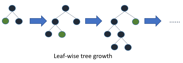
Building the tree leaf-wise results in faster convergence, but may lead to overfitting if the parameters are not tuned accordingly. Important parameters for controlling the tree building are:

• num_leaves: the number of leaf nodes to use. Having a large number of leaves will improve accuracy, but will also lead to overfitting.
• min_child_samples: the minimum number of samples (data) to group into a leaf. The parameter can greatly assist with overfitting: larger sample sizes per leaf will reduce overfitting (but may lead to under-fitting).
• max_depth: controls the depth of the tree explicitly. Shallower trees reduce overfitting.

Tuning for imbalanced data

The simplest way to account for imbalanced or skewed data is to add a weight to the positive class examples:

• scale_pos_weight: the weight can be calculated based on the number of negative and positive examples: sample_pos_weight = number of negative samples / number of positive samples.

Tuning for overfitting

In addition to the parameters mentioned above the following parameters can be used to control overfitting:

• max_bin: the maximum numbers bins that feature values are bucketed in. A smaller max_bin reduces overfitting.
• min_child_weight: the minimum sum hessian for a leaf. In conjuction with min_child_samples, larger values reduce overfitting.
• bagging_fraction and bagging_freq: enables bagging (subsampling) of the training data. Both values need to be set for bagging to be used. The frequency controls how often (iteration) bagging is used. Smaller fractions and frequencies reduce overfitting.
• feature_fraction: controls the subsampling of features used for training (as opposed to subsampling the actual training data in the case of bagging). Smaller fractions reduce overfitting.
• lambda_l1 and lambda_l2: controls L1 and L2 regularization.

Tuning for accuracy

Accuracy may be improved by tuning the following parameters:

• max_bin: a larger max_bin increases accuracy.
• learning_rate: using a smaller learning rate and increasing the number of iterations may improve accuracy.
• num_leaves: increasing the number of leaves increases accuracy with a high risk of overfitting.

A great overview of both XGBoost and LightGBM parameters, their effect on various aspects of the algorithms and how they relate to each other is available here.

Resources

1. LightGBM project: https://github.com/Microsoft/LightGBM
2. LightGBM paper: https://www.microsoft.com/en-us/research/wp-content/uploads/2017/11/lightgbm.pdf
3. Documentation: https://lightgbm.readthedocs.io/en/latest/index.html
4. Parameters: https://lightgbm.readthedocs.io/en/latest/Parameters.html
5. Parameter explorer: https://sites.google.com/view/lauraepp/parameters